
Application report
FE model validation using scanning vibrometry
A joint study byOptomet GmbH and Siemens Digital Industries Software


Measure natural frequencies, damping and mode shapes without contact and compare them with simulation results.
A finite element (FE) model is intended to predict how a physical component vibrates. In FE model validation the comparison with measured data shows how well it does so. In a joint study by Optomet and Siemens Digital Industries Software, a scanning vibrometer from the SMART series measures a clamped plate at 208 points. SMART Lab links the measurement to the model geometry. Relative frequency deviations remain below 1.6 % for seven correlated mode pairs.
FE model validation requires spatially dense measurement data
Lightweight and flexible aerospace components need to behave predictably in service. This requires natural frequencies, damping and mode shapes to be represented reliably in the structural model. This is particularly important for flutter analyses: during flutter, the interaction between aerodynamic forces, elasticity and inertia can cause vibrations to grow through self-excitation and threaten the structure.
Optomet and Siemens Digital Industries Software investigated a measurement workflow in Leuven using a plate clamped at one end. It serves as a simplified laboratory analogue for bending-dominated aerospace components such as control surfaces. The study assesses how well the FE model represents their structural dynamics. It is not yet a flutter test.
Measurement points and calibration link the model and test object
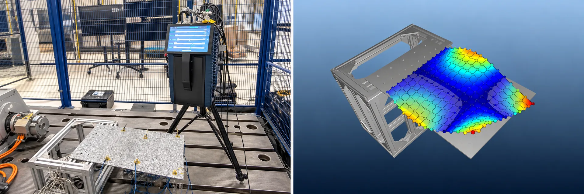
SMART Lab uses the imported structural geometry as the spatial reference for the measurement. A boundary shape is created on its surface and populated with an equidistant grid of measurement points. This is possible on both flat and complex, curved surfaces.
Two steps to a digital measurement setup
First, the model geometry is aligned with the image captured by the integrated 4K camera. An algorithm-supported process matches calibration markers in the camera image with those in the 3D model. Automatic laser calibration then uses these reference points to determine the precise position of the test object relative to the laser beam.
This creates a digital twin of the measurement setup that links the physical test object, model geometry, camera image and laser position within a common spatial reference. This reduces manual mapping effort between measurement and simulation and the need for additional interpolation.
From scan planning to data export
Import the model
The structural geometry is loaded into SMART Lab as the spatial reference.
Define measurement points
An equidistant grid of measurement points is generated within the boundary shape.
Calibrate the setup
The camera image and model are aligned, followed by automatic laser calibration.
Measure vibrations
The vibrometer scans the measurement points while synchronously recording the reference channels.
Visualize responses
Operational deflection shapes can be extracted from the frequency response functions and visualized on the model.
Identify modes
Experimental modal analysis identifies natural frequencies, damping and mode shapes in SMART Lab or external software.
Correlate data
Frequency response functions and geometry are exported in UFF, ATFX, MAT or HDF5 formats. In this study, further processing and comparison are performed in Simcenter 3D.
208 measurement points on a clamped plate
A scanning laser Doppler vibrometer (SLDV) from the SMART series is positioned in front of the plate and measures its motion perpendicular to the observed surface, known as out-of-plane motion. A uniaxial shaker excites the plate. At the excitation point, a force sensor measures the dynamic force actually transmitted into the structure. Accelerometers provide additional pointwise reference measurements.
The vibrometer generates the excitation signal itself and synchronously records the optical measurement data and reference channels. The applied force and structural response are thus available together for calculating frequency response functions.
Test parameters
- Test object
- Flat plate, rigidly clamped along one edge
- Measurement system
- Optomet SMART series scanning laser Doppler vibrometer and SMART Lab
- Excitation
- Uniaxial shaker, chirp from 5 to 500 Hz, signal duration 2 s, signal generator sample rate 14 kHz
- Measurement grid
- 208 measurement points with 30 mm spacing
- Data acquisition
- Velocity measurement range 50 mm/s, measurement frequency range 2 kHz, sample rate 12 kHz
- Measurement duration per point
- Four blocks of 2 s each; 1 s delay between blocks to allow vibrations from previous excitations to fade
- Measured and reference quantities
- Vibration velocity and displacement; synchronously recorded acceleration, applied force and excitation signal
Frequency response functions reveal the vibration response
For each of the 208 measurement points, a frequency response function (FRF) is calculated from the vibration velocity and applied force. The magnitude averaged over all points shows the dynamic response within the investigated frequency range. The black lines in the diagram indicate the natural frequencies subsequently identified by modal analysis.
The four visualizations show selected operational deflection shapes directly on the model geometry. At higher frequencies, the deformation patterns become more spatially complex. The dense measurement grid makes these differences visible.
Modal analysis identifies seven mode shapes
Experimental modal analysis of the frequency response functions over the excitation range of 5 to 500 Hz is performed. A stabilization diagram helps distinguish physical structural modes from numerical or noise-related poles. This involves checking whether frequency, damping, and mode-shape behavior remain consistent as the model order increases.
Measured natural frequencies and damping
| Natural Frequency (Hz) | Modal Damping (%) | |
|---|---|---|
| Mode 1 | 16.09 | 0.59 |
| Mode 2 | 46.42 | 0.55 |
| Mode 3 | 98.68 | 0.10 |
| Mode 4 | 159.28 | 0.01 |
| Mode 5 | 189.73 | 0.10 |
| Mode 6 | 278.62 | 0.77 |
| Mode 7 | 320.12 | 0.10 |
The table lists the seven selected modes with natural frequencies ranging from 16.09 to 320.12 Hz and their modal damping. The complex mode shapes shown below retain amplitude and phase information. For the subsequent correlation with the FE results, the experimental mode shapes were converted to real-valued mode shapes and scaled to unit modal mass.
Measured and FE model frequencies show good agreement
The numerical model includes both the plate and the supporting fixture. The interface between them represents the clamped boundary condition used in the experimental setup. This allows the influence of the fixture to be included in the numerical modal analysis; the plate is not considered as an isolated structure. Simcenter 3D calculates the natural frequencies and mode shapes.
Measured and calculated natural frequencies
| Exp. Frequency (Hz) | Num. Mode | Num. Frequency (Hz) | Δf (%) | |
|---|---|---|---|---|
| Exp. Mode 1 | 16.09 | 1 | 16.08 | −0.11 |
| Exp. Mode 2 | 46.42 | 2 | 46.74 | +0.69 |
| Exp. Mode 3 | 98.68 | 3 | 98.83 | +0.14 |
| Exp. Mode 4 | 159.28 | 6 | 161.82 | +1.59 |
| Exp. Mode 5 | 189.73 | 8 | 186.98 | −1.45 |
| Exp. Mode 6 | 278.62 | 9 | 279.31 | +0.25 |
| Exp. Mode 7 | 320.12 | 10 | 321.40 | +0.40 |
The MAC matrix compares spatial mode shapes
Similar natural frequencies alone do not establish whether measurement and simulation describe the same deformation patterns. The Modal Assurance Criterion (MAC) therefore assesses the agreement between experimental and numerical mode shapes and helps identify corresponding mode pairs.
High MAC values for the correlated pairs indicate similar mode shapes. Low values between unrelated modes support their separation. In addition, a direct visual comparison shows that the model reproduces the main deformation characteristics of the selected experimental modes.
Boundary conditions and measurement direction limit the comparison
Surface geometry and the numerical mesh are not the same
SMART Lab can use surface geometry data for scan definition. FE simulation additionally requires appropriate elements, material properties and boundary conditions. The surface representation used for optical measurement planning is therefore not necessarily identical to the numerical mesh. Mesh topology and modelling assumptions remain important when interpreting the results.
A single measurement direction does not capture every motion
The experiment captures motion in a single measurement direction on the observed side of the plate. This is sufficient to characterize its dominant bending behavior. The FE model, however, describes the full three-dimensional displacement field. Modes with pronounced in-plane components or local three-dimensional deformation patterns may therefore show reduced correlation with the measured data.
Future investigations using 3D scanning vibrometry could also capture these motion components and improve correlation for more complex or larger components.
Measurement data support model updating and further testing
The measured frequency response functions, associated geometry and identified modes provide a basis for model updating, which involves targeted adjustments to the numerical model based on experimental results. The value lies in the consistent spatial link between scan definition, calibration, measurement and modal correlation.
The long-term objective is to support investigations of flutter and modal coupling. In so-called dry wind tunnel tests, aerodynamic effects are represented without physical airflow, for example through actuator forces, equivalent loads, or the combination of measured structural frequency response functions with calculated aerodynamic models. The aim is to reduce experimental complexity, cost and development risk. This requires reliable structural data. The present study provides a preparatory step toward this objective.
Not all measured frequency response functions need to be used in a subsequent reduced-order aeroelastic model. The spatially dense data can support the selection of suitable measurement coordinates, reduce interpolation uncertainty, and verify that the reduced representation captures relevant deformation patterns and modal coupling.
Smart measurement systems for your testing needs
Laser Doppler vibrometers and SMART Lab combine non-contact vibration measurement with model-based analysis. The appropriate configuration depends on the component geometry and the required measurement directions. The experiment described here used a SMART series scanning system with a single measurement direction.
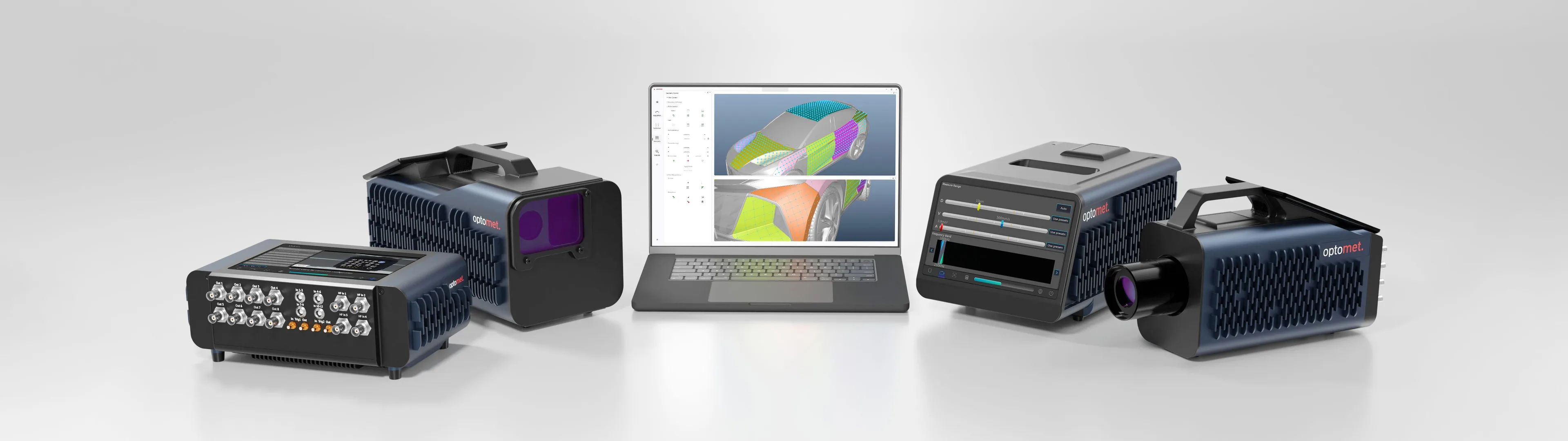
SMART Lab Software
Measurement planning on the model geometry, calibration, data acquisition, modal analysis and export.
View product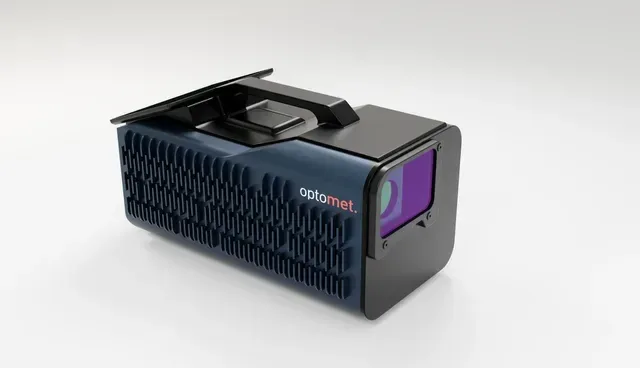
SMART Scan+
Full-field vibration measurement in a single measurement direction using a scanning laser Doppler vibrometer.
View product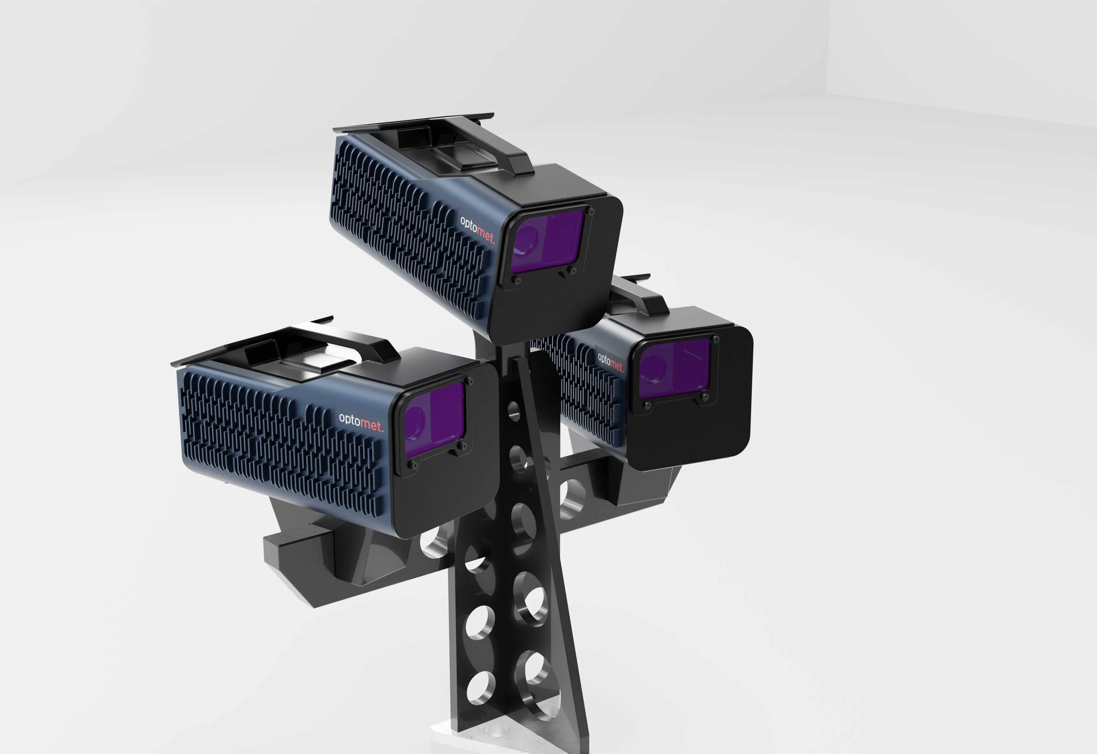
SMART 3D-Scan
Three-dimensional measurement for applications requiring additional motion directions to be captured.
View productLooking to correlate an FE model with measurement data? Discuss your component, the frequency range of interest and the required measurement directions with us.
Experimental setup, results and figures in the original paper
This application report is based on the paper “Experimental validation of FE models using FE-model-based scanning laser Doppler vibrometry” by Tom Burmeister, Davide Mastrodicasa and other authors from Optomet and Siemens Digital Industries Software. The paper’s results were presented as a scientific poster at ISMA 2026, held from 7 to 9 September. The original English text provides a more detailed explanation of the methodology and scientific context.
The download contains the final 14-page version of the paper accepted for ISMA 2026, including all figures, results tables and references.