
Application report
3D vibration analysis for turbine blades and blisks

Measure natural frequencies, vibration shapes and dynamic strains without contact and visualize them directly on the 3D model.
Laser Doppler vibrometers from Optomet measure vibrations on turbine and compressor blades precisely and without contact, even under varying load and temperature conditions. With the SMART series, you can capture motion in one or three spatial directions. Measurements from multiple perspectives capture the turbine blade from all sides. The results are visualized directly on the 3D model. This report presents the measurement workflow for a turbine blade and explains how the data can be used to analyze vibration shapes, compare results with simulations and test components.
Why measure turbine component vibrations across the full surface in three dimensions?
Fluctuating pressure fields, thermal loads and repeated excitation place turbine blades under stress. When an excitation frequency is close to a natural frequency, large vibration amplitudes can occur. These produce dynamic strains and can cause critical stresses in the material. Considering static loads alone is therefore insufficient for design. Three-dimensional vibrations and the number of load cycles are also crucial.
Why a few sensor points are often not enough
Low-frequency, global vibration shapes can often be identified using just a few measurement positions. As frequency increases, however, spatial vibration patterns typically become more complex. Local maxima, nodal lines and coupled motions can occur between widely spaced sensor positions and therefore remain undetected.
Measurements with individual bonded sensors have their limitations: they capture only selected positions and can affect the vibration behavior of lightweight turbine blades.
High measurement point density for local mode shapes
Scanning vibrometers capture hundreds to thousands of freely definable measurement positions. The measurement grid can be tailored to the geometry, the expected spatial wavelength and the relevant regions of the FE model. This also reveals localized mode shapes at higher frequencies.
Conventional sensors
- A small number of measurement positions can identify global modes. Local maxima, nodal lines and coupled motion often go undetected between sensors.
- Transducers, adhesive and cables alter the behavior of lightweight or thin-walled turbine blades.
- Components require wiring and preparation.
- Transducers cannot be attached to glowing-hot surfaces and can come loose at large amplitudes.
Scanning laser vibrometry
- Hundreds to thousands of freely definable measurement points, tailored to the geometry, expected wavelength and FE model. This also reveals local modes at higher frequencies.
- No sensor mass or cable forces: natural frequencies and mode shapes remain unaffected.
- Measurements can be taken on almost any surface without preparation; reflective tape is generally unnecessary.
- Even glowing-hot components and extremely large amplitudes can be measured. No other vibration measurement principle achieves a dynamic range of 220 dB and a measurement range of 0–50 MHz.
Measurement workflow: from the 3D model to measurement
To capture localized mode shapes as well, measurement points are defined directly on the 3D geometry. The CAD model or finite element model (FE model) provides a shared coordinate system for this purpose. Measurement points, measurement directions and results can thus be linked unambiguously.
Measurement preparation starts with the CAD or FE model, before working with the camera image. Measurement points are defined on this digital geometry at the locations needed for subsequent comparison with the simulation.
Define measurement points
Measurement areas and point density are defined on the 3D geometry. Measurement points can be generated automatically and then adjusted individually. This creates a 360° measurement grid with uniform spacing, even on curved surfaces. Nodes from the FE model can be used directly as measurement points.
Align the camera image and 3D model
Geometric calibration takes place in two steps. First, an algorithm automatically aligns the 3D geometry with the camera image of the physical component.
Align the lasers
Defined calibration points from the 3D model are then mapped onto the physical component. The lasers automatically align with these points, establishing their spatial relationship to the turbine blade. This takes a few minutes per scanning head. A complete 3D setup can be aligned in approximately 3 to 10 minutes.
Create a digital representation
The turbine blade, measurement heads, lines of sight and measurement points now share a common coordinate system.
Excite the blade
The turbine blade is excited using an impact hammer, an automated modal hammer, a shaker or acoustic excitation. A reference signal enables the calculation of frequency response functions (FRF). In the example shown, the load cell in the modal hammer provides this signal.
Monitor data in real time
During measurement, SMART Lab displays time-domain data, the reference signal, measurement progress and animations of the points already measured. This allows signal quality and settings to be checked early on.
Analyze frequency responses and vibration shapes
Using the measurement and reference signals, SMART Lab calculates the frequency response functions (FRF) for all measurement points and directions. For any selected frequency, the corresponding vibration shape can be animated directly on the component model, including at resonance frequencies. Analysis is possible in the spatial directions x, y and z as well as along the laser directions u, v and w, in each case relative to the reference signal.
Example: 3D full-body modal analysis of a turbine blade
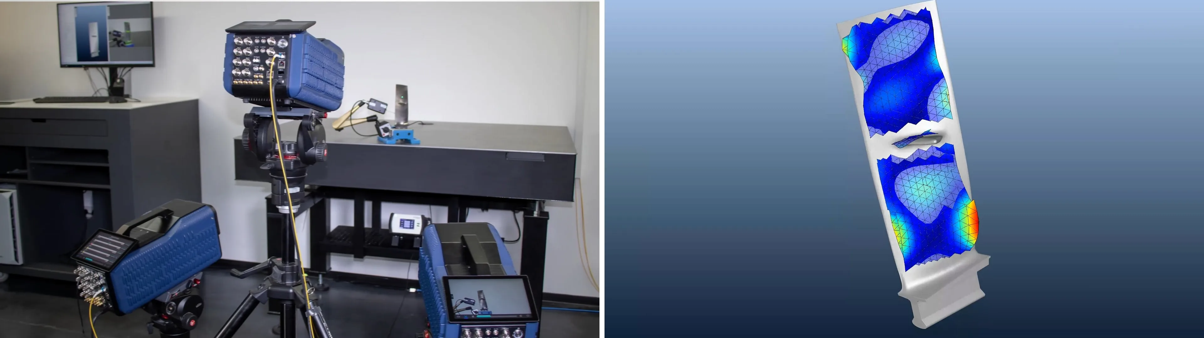
A demonstration measurement illustrates the workflow using an approximately 30 × 10 cm turbine blade. The turbine blade was clamped and excited using an automated modal hammer. Three SMART Scan+ operated as a synchronized 3D system. They captured the visible surfaces from six calibrated perspectives around the turbine blade.
- Test object
- Clamped turbine blade, approx. 30 × 10 cm
- Measurement system
- 3 × SMART Scan+ configured as a SMART 3D-Scan / full-body 3D setup
- Perspectives
- 6 geometrically calibrated views
- Measurement points
- Around 800 points on the 3D model
- Frequency range
- Up to approximately 30 kHz
- Excitation
- Hammer excitation with a reference signal
- Measurement time
- Approx. 2 s per point; around 27 min of data acquisition
- Calibration time
- Approx. 3 min per perspective; around 18 min in total
- Total duration
- Around 45 min after setup, excluding initial setup time
The result: vibration shapes across all surfaces and in three directions
Validate FE models and determine dynamic strain
Visualize dynamic strain
Using the spatially resolved 3D motion of neighboring measurement points, SMART Lab also calculates dynamic strain. This reveals both the resonance frequencies and the locations where strain is particularly high. Non-contact measurement complements conventional strain gauges (DMS) and can reduce the number required for full-field investigations.
Compare measurements directly with simulations
Since the measurement points are defined on the 3D model, it is possible to compare measurements and simulations at the same locations. Higher-frequency and localized vibration shapes, in particular, reveal how accurately the model's material parameters, boundary conditions, and geometric details represent reality. The data support the validation of FE models in several ways:
- Determine natural frequencies and modal parameters experimentally
- Compare global and local vibration shapes
- Position measurement points precisely at FE nodes and in critical regions
- Export measurement and geometry data for CAE and modal analysis software
- Support model updating with experimental data at high spatial resolution
Mistuning, component comparison, and End-of-Line testing
Small differences in geometry, material, coating, or manufacturing alter the natural frequencies and vibration shapes of individual turbine blades. Such variations between nominally identical turbine blades are known as Mistuning and, with reproducibly defined measurement positions, different components, individual turbine blades on a blisk, and conditions before and after manufacturing or repair can be compared:
- Comparison of natural frequencies, frequency responses, and selected vibration shape metrics
- Detection of variations between nominally identical turbine blades
- Testing after manufacturing, coating, or repair
- Reuse of defined measurement positions and test procedures
- Customer-specific pass/fail assessment based on approved limits
SMART Multi-Fiber: simultaneous measurements, flexible configuration
Production testing does not always require a full scan with around 800 points. Depending on the defect being targeted and the metrics required, a few carefully selected measurement positions may be sufficient. Measuring several points simultaneously can reduce testing time.
For this purpose, SMART Multi-Fiber complements the scanning systems. Up to four Fiber Heads per unit take synchronized, phase-consistent measurements. Multiple systems can be linked to form a larger measurement network.
Depending on the configuration, autofocus measurement heads, compact measurement heads or 3D-Fiber-Heads are available. They can be used for reference, transfer path and comparative measurements, including in confined spaces or under demanding thermal conditions. Single-point 3D measurements are also possible.
Smart measurement systems for your testing needs


SMART 3D-Scan
3D scanning measurements: complete motion vectors, a basis for strain analysis
View product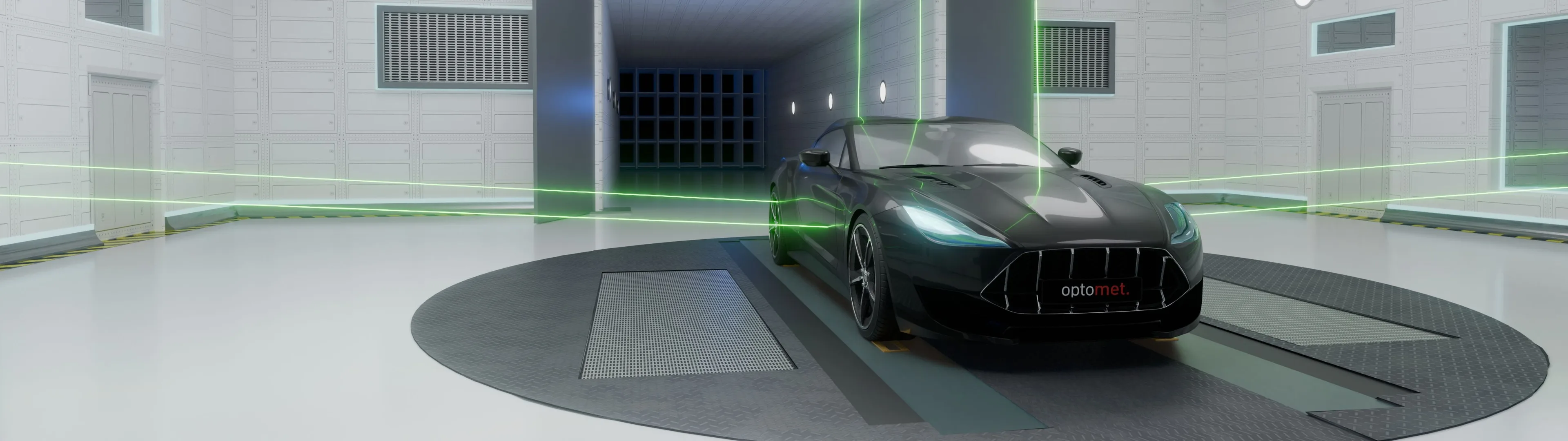
SMART Full Body
Multiple perspectives: capture complex turbine blades from all sides in a single project
View product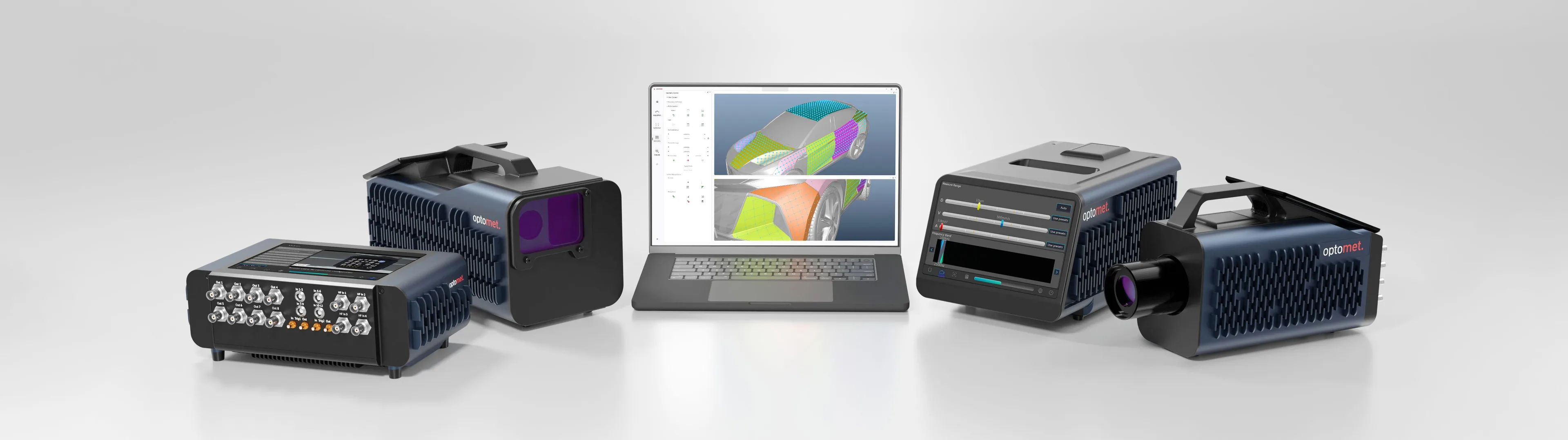
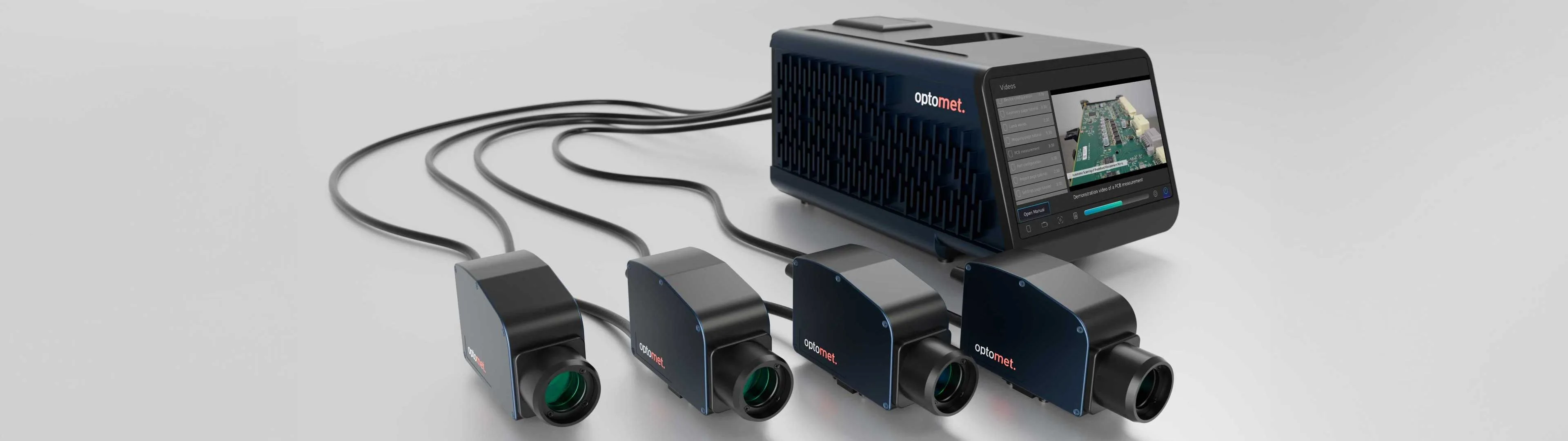
SMART Multi-Fiber
Simultaneous multipoint measurements: references, fixed measurement points, single-point 3D measurements
View productFrequently asked questions
Why are three vibrometers needed for a 3D measurement?
Each laser beam measures velocity along its measurement direction. Three synchronized beams from known geometric directions make it possible to determine motion in all three spatial directions.
How are measurement points mapped to the FE model?
Measurement points are defined directly on the imported 3D geometry. Calibrating the camera and lasers aligns the physical component and the vibrometers within the same coordinate system.
Is stitching required for full-body measurements?
No. Additional viewpoints are calibrated to the same 3D model. All points and results are therefore already in the shared project coordinate system.
Can measurements be performed on hot surfaces?
Yes, provided the measurement head and optical path are protected and sufficient backscattered light is available. Feasibility depends on the test setup and surface.
Can testing be automated?
Measurement sequences, measurement positions and customer-specific limits can be configured for recurring tests. Handling and process integration can be implemented in collaboration with automation partners as needed.
Which measurement strategy suits your application?
How many measurement points are needed? Which frequency range and excitation suit the task? And is a 1D measurement sufficient, or is a SMART 3D-Scan required? For an initial assessment, it helps us to know the component type, approximate dimensions, expected frequency range, test conditions and desired outcome.